Tensorflow 2+ with Keras Images and CNN
https://www.tensorflow.org/tutorials/images/cnn
#============================================ #STEP 1 Import TEnsroflow and keras import tensorflow as tf
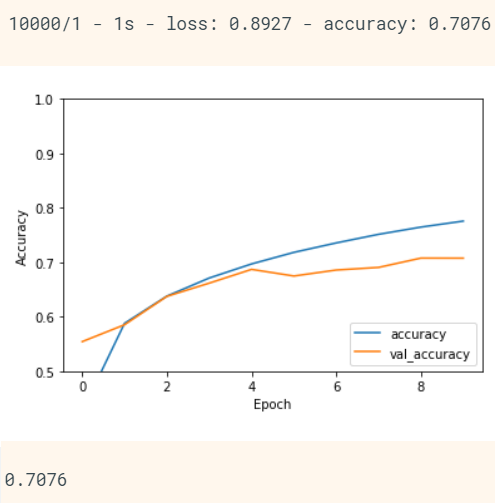
#=============================================================== #STEP 6- plot the accuracy plt.plot(history.history['accuracy'], label='accuracy') |
 #============================================================
#STEP 3 - start creating CNN model with setup of convolution layers
#Create the CNN model-
#============================================================
#STEP 3 - start creating CNN model with setup of convolution layers
#Create the CNN model-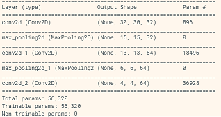 #=======================================================
#STEP 4 - complete CNN layers to add fully connected layers leading to final decision layer
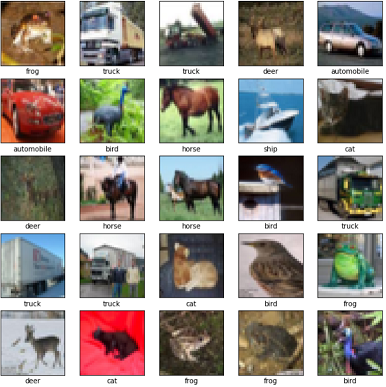
# note CIFAR has 10 output classes
# input to first fully connect layer is the output from
#=======================================================
#STEP 4 - complete CNN layers to add fully connected layers leading to final decision layer
# note CIFAR has 10 output classes
# input to first fully connect layer is the output from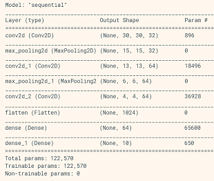 #================================================================
#STEP 5- setup optimizer &loss & accuracy AND Train the model
model.compile(optimizer='adam',
#================================================================
#STEP 5- setup optimizer &loss & accuracy AND Train the model
model.compile(optimizer='adam',